What you'll be able to do本章學習成果
- Use multi-constant equations of state to relate $p$, $v$, $T$.運用多常數狀態方程式建立 $p$、$v$、$T$ 之間的關係。
- Exploit exact differentials and the Maxwell relations to get entropy from $p$–$v$–$T$ data.利用全微分與麥克斯韋關係式,從 $p$–$v$–$T$ 資料求得熵。
- Apply the Clapeyron equation across phase change, and evaluate $\Delta u$, $\Delta h$, $\Delta s$ for single phases.將克拉佩龍方程式應用於相變,並計算單相的 $\Delta u$、$\Delta h$、$\Delta s$。
- Use generalized enthalpy and entropy departure charts for real gases.使用廣義焓與熵偏差圖表處理真實氣體。
Key equations重要公式
Equations of state狀態方程式
An accurate $p$–$v$–$T$ relationship is the foundation for every other property. Beyond the ideal gas, two-constant cubic equations add the molecular effects the ideal model ignores — finite molecular volume and intermolecular attraction:精確的 $p$–$v$–$T$ 關係式是所有其他性質的基礎。在理想氣體之外,兩常數立方型方程式加入了理想模型所忽略的分子效應——有限分子體積與分子間吸引力:
The constants $a$ and $b$ come from the critical-point data. Multi-constant forms (Beattie–Bridgeman, Benedict–Webb–Rubin) extend accuracy to high density. The virial equation expands $Z$ as a power series in $1/v$.常數 $a$ 與 $b$ 由臨界點資料決定。多常數形式(Beattie–Bridgeman、Benedict–Webb–Rubin)可將準確度延伸至高密度。維里方程式則以 $1/v$ 的冪級數展開 $Z$。
Equation-of-state p–v plotter狀態方程式 p–v 繪圖器
Plot isotherms for CO₂ and compare the ideal gas with the van der Waals and Redlich–Kwong equations. Above the critical temperature the curves are smooth and monotonic; drop below $T_c = 304$ K and the cubic equations develop the famous van der Waals loop — the equation's attempt to describe the two-phase region. Toggle each model and watch where the ideal gas diverges.繪製 CO₂ 的等溫線,比較理想氣體、范德瓦耳斯方程式與 Redlich–Kwong 方程式。在臨界溫度以上,曲線平滑單調;低於 $T_c = 304$ K 時,立方型方程式會出現著名的范德瓦耳斯迴圈——方程式試圖描述兩相區的結果。切換各模型,觀察理想氣體在哪裡開始偏離。
Partial-derivative relations偏微分關係式
Because properties are continuous point functions with exact differentials, their mixed second derivatives are equal. For $z = z(x,y)$ with $dz = M\,dx + N\,dy$, exactness requires:由於性質是具有全微分的連續點函數,其混合二階偏導數相等。對於 $z = z(x,y)$,若 $dz = M\,dx + N\,dy$,全微分條件要求:
Two more identities do heavy lifting: the reciprocity relation $(\partial x/\partial y)_z = 1/(\partial y/\partial x)_z$ and the cyclic relation $(\partial x/\partial y)_z(\partial y/\partial z)_x(\partial z/\partial x)_y = -1$.另兩個恆等式也極為重要:倒數關係 $(\partial x/\partial y)_z = 1/(\partial y/\partial x)_z$ 以及循環關係 $(\partial x/\partial y)_z(\partial y/\partial z)_x(\partial z/\partial x)_y = -1$。
Maxwell relations麥克斯韋關係式
Applying exactness to the four Gibbs equations (built from $du$, $dh$, and the Helmholtz $\psi = u - Ts$ and Gibbs $g = h - Ts$ functions) yields the Maxwell relations:將全微分條件應用於四個吉布斯方程式(由 $du$、$dh$、亥姆霍茲函數 $\psi = u - Ts$ 與吉布斯函數 $g = h - Ts$ 構成),即可導出麥克斯韋關係式:
Two everyday ideas are hiding in these definitions.這兩個定義其實藏著兩個生活化的概念。
1. "Free energy" = the spendable part of your energy. Picture the internal energy $u$ as a bank balance. Not all of it is withdrawable — a chunk is "frozen," tied up in the random thermal jiggling (entropy) at temperature $T$. That frozen, un-spendable amount is exactly $Ts$. What's left, $u - Ts$, is the part you can actually withdraw as useful work — the free energy $\psi$. Gibbs $g = h - Ts$ is the same idea, just starting from enthalpy $h$ (which already includes the work to push back the surrounding pressure).1.「自由能」=能量中可動用的部分。把內能 $u$ 想成銀行存款。並非全部都能提領——有一部分被「凍結」,被溫度 $T$ 下的隨機熱運動(熵)綁住了。這筆被凍結、無法動用的能量正好是 $Ts$。剩下的 $u - Ts$,才是你真正能以有用功提領出來的部分——即自由能 $\psi$。吉布斯 $g = h - Ts$ 是同樣的概念,只是從焓 $h$ 出發($h$ 已包含為了推開周圍壓力所需的功)。
2. We rewrite energy using the knobs we can actually turn. In the lab you set temperature (a water bath, a thermostat) and pressure (open to the atmosphere, a weighted piston) — there is no "entropy dial." Yet $u$ and $h$ are naturally functions of entropy. Subtracting $Ts$ is the move that swaps entropy for temperature as the variable you hold fixed. The result: $\psi$ fits a constant-temperature, fixed-volume system (a sealed rigid tank in a water bath), and $g$ fits a constant-temperature, constant-pressure one (anything sitting open on the bench at room temperature — which is why $g$ governs melting, boiling, and chemical reactions).2. 我們用「實際能轉動的旋鈕」改寫能量。在實驗室裡,你能設定的是溫度(水浴、恆溫器)與壓力(對大氣開放、加重活塞)——並沒有「熵旋鈕」。但 $u$ 與 $h$ 天生是熵的函數。減去 $Ts$ 這個動作,恰好把熵換成溫度作為你固定的變數。結果是:$\psi$ 適用於定溫、定容的系統(水浴中密封的剛性容器),$g$ 適用於定溫、定壓的系統(任何在室溫下開放置於檯面上的系統——這正是 $g$ 主宰熔化、沸騰與化學反應的原因)。
For the curious: the "cancel the $T\,ds$ term" algebra in the derivation below is just the formal version of this swap — entropy out, temperature in. Mathematicians call it a Legendre transform.想深入者:下方推導中「消去 $T\,ds$ 項」的代數,只是這個替換的正式版本——換掉熵、換入溫度。數學上稱為勒壤得轉換。
Derivation推導 From the Gibbs equations, step by step由吉布斯方程式逐步推導 ›
Step 1 — The two fundamental differentials. Combine the first law $du = \delta q - \delta w$ with the reversible second law ($\delta q = T\,ds$) and boundary work ($\delta w = p\,dv$):步驟 1 — 兩個基本微分式。將第一定律 $du = \delta q - \delta w$ 與可逆第二定律($\delta q = T\,ds$)及邊界功($\delta w = p\,dv$)結合:
$$ du = T\,ds - p\,dv $$
Differentiate the definition $h = u + pv$ and substitute: $dh = du + p\,dv + v\,dp$, so對定義 $h = u + pv$ 微分並代入:$dh = du + p\,dv + v\,dp$,故
$$ dh = T\,ds + v\,dp $$
Step 2 — The Helmholtz and Gibbs functions. Define $\psi = u - Ts$ (Helmholtz) and $g = h - Ts$ (Gibbs). Differentiate each and substitute the results of Step 1:步驟 2 — 亥姆霍茲與吉布斯函數。定義 $\psi = u - Ts$(亥姆霍茲)與 $g = h - Ts$(吉布斯)。對兩者微分,並代入步驟 1 的結果:
$$ d\psi = du - T\,ds - s\,dT = (T\,ds - p\,dv) - T\,ds - s\,dT = -s\,dT - p\,dv $$
$$ dg = dh - T\,ds - s\,dT = (T\,ds + v\,dp) - T\,ds - s\,dT = -s\,dT + v\,dp $$
These four results — for $du$, $dh$, $d\psi$, $dg$ — are the Gibbs equations.這四個結果——$du$、$dh$、$d\psi$、$dg$——即為吉布斯方程式。
Step 3 — Apply the exactness condition. Each Gibbs equation has the form $dz = M\,dx + N\,dy$, and because $z$ is a property its differential is exact: $\left(\frac{\partial M}{\partial y}\right)_x = \left(\frac{\partial N}{\partial x}\right)_y$. Reading off $M$ and $N$ from each equation gives the four Maxwell relations directly:步驟 3 — 套用全微分條件。每個吉布斯方程式皆為 $dz = M\,dx + N\,dy$ 的形式;由於 $z$ 是性質,其微分為全微分:$\left(\frac{\partial M}{\partial y}\right)_x = \left(\frac{\partial N}{\partial x}\right)_y$。從每式讀出 $M$ 與 $N$,即可直接得到四個麥克斯韋關係式:
$$ \begin{aligned} du = T\,ds - p\,dv \;&\Rightarrow\; \left(\tfrac{\partial T}{\partial v}\right)_s = -\left(\tfrac{\partial p}{\partial s}\right)_v \\[4pt] dh = T\,ds + v\,dp \;&\Rightarrow\; \left(\tfrac{\partial T}{\partial p}\right)_s = \left(\tfrac{\partial v}{\partial s}\right)_p \\[4pt] d\psi = -s\,dT - p\,dv \;&\Rightarrow\; \left(\tfrac{\partial s}{\partial v}\right)_T = \left(\tfrac{\partial p}{\partial T}\right)_v \\[4pt] dg = -s\,dT + v\,dp \;&\Rightarrow\; \left(\tfrac{\partial s}{\partial p}\right)_T = -\left(\tfrac{\partial v}{\partial T}\right)_p \end{aligned} $$
Entropy can't be measured directly. The Maxwell relations express its derivatives entirely in terms of $p$, $v$, $T$ — quantities you can measure. This is exactly how property tables convert lab measurements into entropy values.熵無法直接量測。麥克斯韋關係式將其偏導數完全以 $p$、$v$、$T$ 表示——這些都是可以量測的量。這正是性質表將實驗量測值轉換為熵值的方式。
The Clapeyron equation克拉佩龍方程式
Applied across a phase change, a Maxwell relation gives the slope of the saturation curve in terms of measurable quantities — the Clapeyron equation:將麥克斯韋關係式應用於相變化,可用可量測量表示飽和曲線的斜率——即克拉佩龍方程式:
Derivation推導 From the Maxwell relation across a phase boundary由跨相界的麥克斯韋關係式推導 ›
Step 1 — Start from a Maxwell relation. The one built from the Helmholtz function relates an entropy derivative to a $p$–$v$–$T$ derivative:步驟 1 — 從麥克斯韋關係式出發。由亥姆霍茲函數導出的那一式,將熵的偏導數與 $p$–$v$–$T$ 偏導數連結:
$$ \left(\frac{\partial s}{\partial v}\right)_T = \left(\frac{\partial p}{\partial T}\right)_v $$
Step 2 — Specialize to the two-phase region. During a phase change, $T$ and $p$ are not independent — the saturation pressure depends on temperature alone. So at fixed $T$ the right-hand derivative is just the saturation-curve slope, a constant across the phase change:步驟 2 — 特化到兩相區。相變化期間,$T$ 與 $p$ 並非獨立——飽和壓力僅取決於溫度。故在固定 $T$ 下,右側偏導數即為飽和曲線斜率,於整個相變化過程中為常數:
$$ \left(\frac{\partial p}{\partial T}\right)_v = \left(\frac{dp}{dT}\right)_{sat} $$
Step 3 — Integrate across the phase change. Holding $T$ (and hence the slope) constant, integrate the Maxwell relation from saturated liquid $f$ to saturated vapour $g$:步驟 3 — 對相變化積分。固定 $T$(因此斜率亦固定),將麥克斯韋關係式由飽和液 $f$ 積分至飽和氣 $g$:
$$ \int_f^g ds = \left(\frac{dp}{dT}\right)_{sat}\!\int_f^g dv \;\;\Rightarrow\;\; s_g - s_f = \left(\frac{dp}{dT}\right)_{sat}(v_g - v_f) $$
Step 4 — Replace the entropy change. A phase change at constant $T$ and $p$ is internally reversible, so $s_g - s_f = \dfrac{h_g - h_f}{T} = \dfrac{h_{fg}}{T}$. Substituting and rearranging gives the Clapeyron equation:步驟 4 — 代換熵變化。定 $T$、定 $p$ 下的相變化為內部可逆,故 $s_g - s_f = \dfrac{h_g - h_f}{T} = \dfrac{h_{fg}}{T}$。代入並整理即得克拉佩龍方程式:
$$ \left(\frac{dp}{dT}\right)_{sat} = \frac{h_{fg}}{T(v_g - v_f)} $$
Step 5 — The Clausius–Clapeyron approximation. Far below the critical point the liquid volume is negligible ($v_g \gg v_f$, so $v_g - v_f \approx v_g$) and the vapour is nearly ideal ($v_g = RT/p$). Then:步驟 5 — 克勞修斯–克拉佩龍近似。在遠低於臨界點處,液體體積可忽略($v_g \gg v_f$,故 $v_g - v_f \approx v_g$),且蒸氣近乎理想($v_g = RT/p$)。於是:
$$ \left(\frac{dp}{dT}\right)_{sat} \approx \frac{h_{fg}}{T(RT/p)} = \frac{p\,h_{fg}}{RT^2} \;\;\Rightarrow\;\; \left(\frac{d\ln p}{dT}\right)_{sat} = \frac{h_{fg}}{RT^2} $$
Integrated (with $h_{fg}$ roughly constant), this is the straight-line $\ln p$ vs $1/T$ relation used in the pressure-cooker / Yushan estimate below.積分後(取 $h_{fg}$ 近似為常數),即得 $\ln p$ 對 $1/T$ 的直線關係,亦即下方壓力鍋 / 玉山估算所用之式。
It lets you get the enthalpy of vaporization $h_{fg}$ from $p$–$v$–$T$ data alone — just the saturation-curve slope and the specific-volume change. With the approximations $v_g \gg v_f$ and ideal-gas vapor ($v_g = RT/p$), it simplifies to the Clausius–Clapeyron equation $d(\ln p)/dT = h_{fg}/(RT^2)$.它讓你僅憑 $p$–$v$–$T$ 資料——飽和曲線斜率與比體積變化——即可求得汽化焓 $h_{fg}$,無需量熱實驗。若取近似 $v_g \gg v_f$ 且蒸氣為理想氣體($v_g = RT/p$),可化簡為克勞修斯–克拉佩龍方程式 $d(\ln p)/dT = h_{fg}/(RT^2)$。


- A pressure cooker runs at about 200 kPa (≈2 atm). Roughly what temperature does the water reach, and why does that cook food so much faster?壓力鍋約在 200 kPa(≈2 atm)下運作。水大約達到什麼溫度?為何這能讓食物煮得快得多?
- On the summit of Yushan (3,952 m) the pressure is only about 63 kPa. Water boils near 87 °C there. Why does an egg take noticeably longer to hard-boil, even though the water is "boiling"?在玉山(3,952 m)山頂,氣壓僅約 63 kPa,水約在 87 °C 沸騰。為何即使水已「沸騰」,水煮蛋仍明顯需要更久才能煮熟?
- Use the Clausius–Clapeyron equation with $h_{fg}=2257$ kJ/kg to estimate the boiling point at 63 kPa, and compare with 87 °C.以克勞修斯–克拉佩龍方程式(取 $h_{fg}=2257$ kJ/kg)估算在 63 kPa 下的沸點,並與 87 °C 比較。
- ≈ 120 °C at 200 kPa. Following the saturation curve up to 2 atm raises the boiling point by about 20 °C. Reaction and heat-transfer rates rise steeply with temperature (a rough rule of thumb: ~2× per 10 °C), so cooking at 120 °C instead of 100 °C can cut times by half or more.200 kPa 下約 120 °C。沿飽和曲線升至 2 atm,沸點約上升 20 °C。反應與熱傳速率隨溫度急遽上升(粗略經驗法則:每 10 °C 約快一倍),故在 120 °C 而非 100 °C 烹煮,時間可縮短一半以上。
- Boiling is not the same as hot enough. "Boiling" only fixes the temperature at the saturation value for the local pressure. At 87 °C the food simply cooks at 87 °C, not 100 °C — the chemistry is slower, so the egg takes longer. Adding more heat just boils the water away faster; it cannot push the temperature past the saturation point.「沸騰」不等於「夠熱」。沸騰只是把溫度固定在當地壓力對應的飽和值。在 87 °C,食物就是以 87 °C 烹煮,而非 100 °C——化學反應較慢,故蛋需更久。加大火力只會讓水更快蒸乾,無法使溫度超過飽和點。
- Estimate. Integrating $d(\ln p)/dT = h_{fg}/(RT^2)$ between the two states gives $\ln(p_2/p_1) = -\dfrac{h_{fg}}{R}\left(\dfrac{1}{T_2}-\dfrac{1}{T_1}\right)$. With $p_1=101.3$ kPa, $T_1=373$ K, $p_2=63$ kPa and $R=0.4615$ kJ/kg·K for water vapour, solving gives $T_2 \approx 361$ K ≈ 88 °C — within a degree of the measured value. The Clausius–Clapeyron approximation works well here.估算。將 $d(\ln p)/dT = h_{fg}/(RT^2)$ 於兩狀態間積分,得 $\ln(p_2/p_1) = -\dfrac{h_{fg}}{R}\left(\dfrac{1}{T_2}-\dfrac{1}{T_1}\right)$。代入 $p_1=101.3$ kPa、$T_1=373$ K、$p_2=63$ kPa 及水蒸氣 $R=0.4615$ kJ/kg·K,解得 $T_2 \approx 361$ K ≈ 88 °C——與實測值僅差約一度。克勞修斯–克拉佩龍近似在此相當準確。
General relations for Δu, Δh, ΔsΔu、Δh、Δs 的一般關係式
The goal of this section is practical: express the changes in the unmeasurable energy properties ($u$, $h$, $s$) entirely in terms of the measurable specific heats ($c_v$, $c_p$) and $p$–$v$–$T$ behaviour. Everything below follows from the two fundamental differentials and the Maxwell relations derived earlier.本節目標很實際:將無法量測的能量性質($u$、$h$、$s$)的變化,完全以可量測的比熱($c_v$、$c_p$)與 $p$–$v$–$T$ 行為表示。以下所有結果都源自先前導出的兩個基本微分式與麥克斯韋關係式。
The two Tds (entropy) equations兩個 Tds(熵)方程式
Choosing $(T,v)$ or $(T,p)$ as the independent pair and expanding $ds$ gives the two central results from which everything else follows:選 $(T,v)$ 或 $(T,p)$ 為獨立變數對並展開 $ds$,得到兩個核心結果,其餘一切由此推得:
Derivation推導 The Tds equationsTds 方程式 ›
Step 1 — Expand $s = s(T,v)$.步驟 1 — 展開 $s = s(T,v)$。
$$ ds = \left(\frac{\partial s}{\partial T}\right)_v dT + \left(\frac{\partial s}{\partial v}\right)_T dv $$
Step 2 — Identify each coefficient. From $c_v = (\partial u/\partial T)_v$ together with $du = T\,ds - p\,dv$ at constant $v$, the first coefficient is $(\partial s/\partial T)_v = c_v/T$. The second is a Maxwell relation, $(\partial s/\partial v)_T = (\partial p/\partial T)_v$. Substituting gives the first $Tds$ equation.步驟 2 — 辨識各係數。由 $c_v = (\partial u/\partial T)_v$ 與定 $v$ 下的 $du = T\,ds - p\,dv$,得第一個係數 $(\partial s/\partial T)_v = c_v/T$。第二個係數即麥克斯韋關係式 $(\partial s/\partial v)_T = (\partial p/\partial T)_v$。代入即得第一個 $Tds$ 方程式。
Step 3 — Repeat with $s = s(T,p)$. Now $(\partial s/\partial T)_p = c_p/T$ (from $c_p = (\partial h/\partial T)_p$ and $dh = T\,ds + v\,dp$), and the Maxwell relation $(\partial s/\partial p)_T = -(\partial v/\partial T)_p$ gives the second $Tds$ equation.步驟 3 — 以 $s = s(T,p)$ 重複。此時 $(\partial s/\partial T)_p = c_p/T$(由 $c_p = (\partial h/\partial T)_p$ 與 $dh = T\,ds + v\,dp$),麥克斯韋關係式 $(\partial s/\partial p)_T = -(\partial v/\partial T)_p$ 則給出第二個 $Tds$ 方程式。
Internal energy change內能變化
Substituting the first $Tds$ equation into $du = T\,ds - p\,dv$:將第一個 $Tds$ 方程式代入 $du = T\,ds - p\,dv$:
The bracket is the internal pressure $(\partial u/\partial v)_T$. For an ideal gas $p = RT/v$ gives $T(\partial p/\partial T)_v = T(R/v) = p$, so the bracket vanishes and $du = c_v\,dT$ — confirming that ideal-gas internal energy depends on temperature alone.括號項即內壓 $(\partial u/\partial v)_T$。對理想氣體,$p = RT/v$ 給出 $T(\partial p/\partial T)_v = T(R/v) = p$,故括號為零,$du = c_v\,dT$——印證理想氣體內能僅與溫度有關。
Enthalpy change焓變化
Substituting the second $Tds$ equation into $dh = T\,ds + v\,dp$:將第二個 $Tds$ 方程式代入 $dh = T\,ds + v\,dp$:
For an ideal gas $v = RT/p$ gives $T(\partial v/\partial T)_p = v$, the bracket vanishes, and $dh = c_p\,dT$. (Once $\Delta u$ or $\Delta h$ is known, the other follows from $\Delta h = \Delta u + \Delta(pv)$.)對理想氣體,$v = RT/p$ 給出 $T(\partial v/\partial T)_p = v$,括號為零,$dh = c_p\,dT$。(已知 $\Delta u$ 或 $\Delta h$ 之一後,另一個可由 $\Delta h = \Delta u + \Delta(pv)$ 求得。)
Entropy change熵變化
Integrating the $Tds$ equations directly gives two equivalent expressions for $\Delta s$ — choose whichever matches your data:直接積分 $Tds$ 方程式,得到 $\Delta s$ 的兩個等價表示式——依手邊資料選用:
The Mayer relation: $c_p - c_v$邁耶關係式:$c_p - c_v$
Equating the two $Tds$ equations links the specific heats to $p$–$v$–$T$ data alone:令兩個 $Tds$ 方程式相等,即將比熱僅與 $p$–$v$–$T$ 資料連結:
Derivation推導 The Mayer relation邁耶關係式 ›
Step 1 — Set the two $Tds$ equations equal. Both equal $ds$, so:步驟 1 — 令兩個 $Tds$ 方程式相等。兩者皆等於 $ds$,故:
$$ \frac{c_v}{T}\,dT + \left(\frac{\partial p}{\partial T}\right)_v dv = \frac{c_p}{T}\,dT - \left(\frac{\partial v}{\partial T}\right)_p dp $$
Solving for $dT$:解出 $dT$:
$$ dT = \frac{T(\partial p/\partial T)_v}{c_p - c_v}\,dv + \frac{T(\partial v/\partial T)_p}{c_p - c_v}\,dp $$
Step 2 — Compare with $T = T(v,p)$. Expanding $dT = (\partial T/\partial v)_p\,dv + (\partial T/\partial p)_v\,dp$ and matching the $dv$ coefficient:步驟 2 — 與 $T = T(v,p)$ 比較。展開 $dT = (\partial T/\partial v)_p\,dv + (\partial T/\partial p)_v\,dp$,比對 $dv$ 係數:
$$ c_p - c_v = T\left(\frac{\partial v}{\partial T}\right)_p\left(\frac{\partial p}{\partial T}\right)_v $$
Step 3 — Remove the awkward derivative with the cyclic relation. The cyclic relation gives $(\partial p/\partial T)_v = -(\partial v/\partial T)_p (\partial p/\partial v)_T$. Substituting:步驟 3 — 以循環關係消去不便的偏導數。循環關係給出 $(\partial p/\partial T)_v = -(\partial v/\partial T)_p (\partial p/\partial v)_T$。代入:
$$ c_p - c_v = -T\left(\frac{\partial v}{\partial T}\right)_p^{\,2}\left(\frac{\partial p}{\partial v}\right)_T $$
Reading the result. Since $(\partial p/\partial v)_T < 0$ for any stable substance and the squared term is positive, $c_p - c_v \ge 0$ always. It vanishes as $T \to 0$, and is zero for a truly incompressible substance — so $c_p = c_v$ for liquids and solids. For an ideal gas, $(\partial v/\partial T)_p = R/p$ and $(\partial p/\partial v)_T = -p/v$, giving the familiar $c_p - c_v = R$.結果解讀。對任何穩定物質 $(\partial p/\partial v)_T < 0$,且平方項為正,故 $c_p - c_v \ge 0$ 恆成立。當 $T \to 0$ 時趨於零;對真正不可壓縮物質為零——故液體與固體有 $c_p = c_v$。對理想氣體,$(\partial v/\partial T)_p = R/p$、$(\partial p/\partial v)_T = -p/v$,得熟知的 $c_p - c_v = R$。
The Joule–Thomson effect & coefficient焦耳–湯姆生效應與係數
Force a real gas through a valve, porous plug, or narrow orifice and — with no heat added and no shaft work done — its temperature changes. This is the Joule–Thomson (throttling) effect. The flow does just enough flow-work on itself that enthalpy is conserved ($h_1 = h_2$), yet temperature need not be: as the gas expands, its molecules move farther apart and spend energy pulling against their mutual attraction, drawing that energy from their own thermal motion — so the gas cools. For an ideal gas there are no intermolecular forces, so $\mu_J = 0$ and throttling leaves the temperature unchanged.將真實氣體強行通過閥門、多孔塞或狹窄孔口——在無熱量加入、無軸功輸出的情況下——其溫度會改變。這就是焦耳–湯姆生(節流)效應。流動對自身所做的流動功恰好使焓守恆($h_1 = h_2$),但溫度未必守恆:氣體膨脹時,分子彼此遠離,需消耗能量對抗分子間吸引力,而這能量取自其自身的熱運動——故氣體冷卻。對理想氣體而言,並無分子間作用力,故 $\mu_J = 0$,節流不改變溫度。
Quantitatively, the temperature change of a real fluid during throttling ($h$ = constant) is the Joule–Thomson coefficient, the slope of constant-enthalpy lines on a $T$–$p$ diagram:定量上,真實流體在節流過程($h$ = 常數)中的溫度變化由焦耳–湯姆生係數描述,即 $T$–$p$ 圖上等焓線的斜率:
Derivation推導 μ in terms of measurable properties以可量測性質表示 μ ›
Step 1 — Start from the general enthalpy differential. From the $\Delta h$ result derived above,步驟 1 — 由一般焓微分式出發。由前面導出的 $\Delta h$ 結果,
$$ dh = c_p\,dT + \left[v - T\left(\frac{\partial v}{\partial T}\right)_p\right]dp $$
Step 2 — Impose constant enthalpy. Throttling is isenthalpic, so set $dh = 0$ and solve for $(\partial T/\partial p)_h$:步驟 2 — 施加定焓條件。節流為等焓過程,故令 $dh = 0$,解出 $(\partial T/\partial p)_h$:
$$ 0 = c_p\left(\frac{\partial T}{\partial p}\right)_h + \left[v - T\left(\frac{\partial v}{\partial T}\right)_p\right] $$
Step 3 — Rearrange. This expresses $\mu_J$ entirely in terms of $c_p$ and $p$–$v$–$T$ data:步驟 3 — 整理。即將 $\mu_J$ 完全以 $c_p$ 與 $p$–$v$–$T$ 資料表示:
$$ \mu_J = \left(\frac{\partial T}{\partial p}\right)_h = \frac{1}{c_p}\left[T\left(\frac{\partial v}{\partial T}\right)_p - v\right] $$
Reading the result. For an ideal gas $v = RT/p$ gives $T(\partial v/\partial T)_p = v$, so $\mu_J = 0$ — throttling cannot change its temperature. For a real gas, the inversion condition $\mu_J = 0$ occurs exactly where $T(\partial v/\partial T)_p = v$; this traces the inversion curve. Inside it $T(\partial v/\partial T)_p > v$ so $\mu_J > 0$ (cooling); outside it $\mu_J < 0$ (heating).結果解讀。對理想氣體,$v = RT/p$ 給出 $T(\partial v/\partial T)_p = v$,故 $\mu_J = 0$——節流無法改變其溫度。對真實氣體,反轉條件 $\mu_J = 0$ 恰好發生於 $T(\partial v/\partial T)_p = v$ 之處,描繪出反轉曲線。曲線內側 $T(\partial v/\partial T)_p > v$,故 $\mu_J > 0$(致冷);外側 $\mu_J < 0$(致熱)。
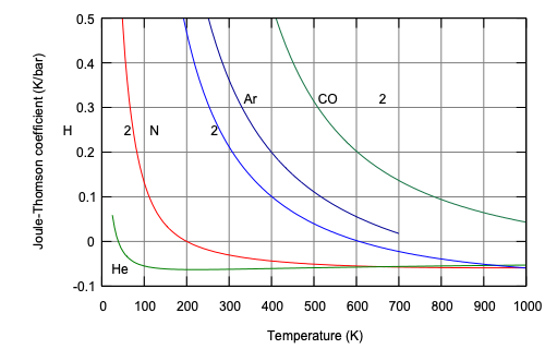
Throttling moves left (decreasing $p$). On the warm side of the inversion line a fluid heats; on the cold side it cools. A cooling effect requires the fluid to be below its maximum inversion temperature — a real constraint for gases like hydrogen and helium whose inversion temperatures sit well below room temperature.節流使狀態向左移動(壓力降低)。在反轉線的熱側,流體升溫;在冷側,流體降溫。要產生冷卻效應,流體必須低於其最高反轉溫度——這對氫氣和氦氣是真實限制,因為它們的反轉溫度遠低於室溫。
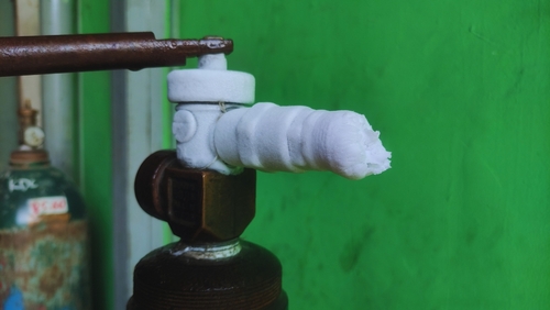
- A spray can also feels cold after prolonged use (we'll demo this in class). Is that the same mechanism as the regulator icing, or something different?長時間使用噴罐後,罐身也會變冷(課堂上會實際示範)。這與調壓器結霜是同一機制,還是不同?
- A high-pressure hydrogen leak warms instead of cooling. Why — and why is that a safety hazard?高壓氫氣洩漏時是升溫而非冷卻。為什麼?為何這是一項安全隱患?
- Which everyday appliance uses this “throttling cools” effect on purpose?哪一種日常家電刻意利用這個「節流致冷」效應?
- Mostly different — the two effects often appear together. A spray can's propellant is usually a liquefied gas (butane/propane), so the dominant cooling is the latent heat of vaporization as the liquid boils off — a phase change, not pure throttling. The escaping vapour then also undergoes Joule–Thomson expansion through the nozzle, adding some J–T cooling. The regulator on a non-liquefied compressed gas (CO₂ above its critical point, air, N₂) is the cleaner, almost-pure J–T case.大多不同——但兩種效應常同時出現。噴罐的推進劑通常是液化氣體(丁烷/丙烷),故主要冷卻來自液體永騰時的永發潛熱——是相變化,而非純節流。逸出的蒸氣隨後也透過噴嘴進行焦耳–湯姆生膨脹,增添部分 J–T 冷卻。而非液化壓縮氣體(超臨界 CO₂、空氣、N₂)的調壓器,則是較純粋的 J–T 案例。
- Hydrogen's maximum inversion temperature (~202 K) is below room temperature. At ambient $T$ it sits on the warm side of the inversion curve, where $\mu_J < 0$, so throttling heats it. A leaking high-pressure H₂ jet can therefore self-heat and ignite — a real hazard in hydrogen handling. (Helium behaves the same way; both must be pre-cooled below their inversion temperature before throttling can liquefy them.)氫的最高反轉溫度(約 202 K)低於室溫。在常溫 $T$ 下,它位於反轉曲線的熱側,$\mu_J < 0$,故節流使其升溫。洩漏的高壓氫氣噴流因而可能自行升溫並點燃——這是氫氣處理的真實危険。(汦氣也是如此;兩者都必須先預冷至反轉溫度以下,節流才能使其液化。)
- The refrigerator and air conditioner. Their expansion valve (or capillary tube) throttles the refrigerant, and the Joule–Thomson cooling is exactly what drops it to the cold-side temperature inside the evaporator. See Refrigeration & Heat Pumps.冰箱與冷氣。其膨脹閥(或毛細管)對冷媒節流,焦耳–湯姆生冷卻正是使其降至蒸發器內冷側溫度的原因。詳見製冷與熱泵。
A short explainer video for the throttling effect:關於節流效應的簡短解說影片:
Watch on YouTube在 YouTube 觀看Enthalpy & entropy departures焓與熵偏差
At high pressure, gases deviate from ideal behavior and $h$ depends on pressure as well as temperature. The difference between the real and ideal-gas value at the same temperature is the enthalpy departure; dividing by $R T_c$ gives the dimensionless departure factor $Z_h$, charted against reduced pressure and temperature. An analogous entropy departure $Z_s$ handles entropy. The real-gas change is then the ideal-gas change (from the tables) corrected by the departures at the two states — the bridge from ideal-gas tables to real-gas reality.在高壓下,氣體偏離理想行為,$h$ 同時依賴壓力與溫度。相同溫度下真實值與理想氣體值之差稱為焓偏差;除以 $R T_c$ 得無因次偏差因子 $Z_h$,以對比壓力和對比溫度繪製成圖。類似的熵偏差 $Z_s$ 處理熵的修正。真實氣體的變化量即為理想氣體變化量(查表所得)加上兩狀態偏差修正——這是從理想氣體表通往真實氣體的橋樑。
Clausius–Clapeyron estimate克勞修斯–克拉佩龍估算
Example範例 Saturation pressure of water at 105 °C水在 105 °C 的飽和壓力 ›
Given: at 100 °C, $p_{sat}=101.3$ kPa and $h_{fg}=2257$ kJ/kg; $R=0.4615$ kJ/kg·K for water.已知:在 100 °C,$p_{sat}=101.3$ kPa,$h_{fg}=2257$ kJ/kg;水的 $R=0.4615$ kJ/kg·K。
Find: the saturation pressure at 105 °C.求:105 °C 時的飽和壓力。
Solution. The Clausius–Clapeyron equation integrates to $$\ln\frac{p_2}{p_1}=\frac{h_{fg}}{R}\left(\frac{1}{T_1}-\frac{1}{T_2}\right)=\frac{2257}{0.4615}\left(\frac{1}{373.15}-\frac{1}{378.15}\right)=0.173.$$ So $p_2=101.3\,e^{0.173}=120\text{ kPa}$ — close to the tabulated 120.8 kPa.解:積分克勞修斯–克拉佩龍方程式得 $$\ln\frac{p_2}{p_1}=\frac{h_{fg}}{R}\left(\frac{1}{T_1}-\frac{1}{T_2}\right)=\frac{2257}{0.4615}\left(\frac{1}{373.15}-\frac{1}{378.15}\right)=0.173。$$ 故 $p_2=101.3\,e^{0.173}=120$ kPa——與表格值 120.8 kPa 相近。
Practice problems練習題
Try each one yourself first, then reveal the solution step by step to check your reasoning.請先自行嘗試,再逐步展開解答核對思路。